

What Is A Data Table In Science
Relational information
Introduction
It'southward rare that a data analysis involves only a single table of data. Typically you have many tables of data, and you must combine them to answer the questions that you lot're interested in. Collectively, multiple tables of data are called relational information considering information technology is the relations, not simply the individual datasets, that are important.
Relations are always defined betwixt a pair of tables. All other relations are built up from this simple idea: the relations of iii or more tables are always a property of the relations betwixt each pair. Sometimes both elements of a pair can exist the same table! This is needed if, for case, you have a table of people, and each person has a reference to their parents.
To work with relational data you need verbs that work with pairs of tables. There are 3 families of verbs designed to work with relational data:
-
Mutating joins, which add together new variables to ane data frame from matching observations in some other.
-
Filtering joins, which filter observations from i information frame based on whether or not they lucifer an observation in the other table.
-
Set operations, which care for observations as if they were set elements.
The nigh common place to detect relational information is in a relational database direction system (or RDBMS), a term that encompasses almost all modernistic databases. If you've used a database before, you've near certainly used SQL. If so, you should find the concepts in this chapter familiar, although their expression in dplyr is a little different. Generally, dplyr is a little easier to utilise than SQL considering dplyr is specialised to do data analysis: it makes common data analysis operations easier, at the expense of making it more difficult to do other things that aren't commonly needed for data analysis.
Prerequisites
We volition explore relational data from nycflights13 using the two-tabular array verbs from dplyr.
nycflights13
We will apply the nycflights13 package to larn most relational data. nycflights13 contains iv tibbles that are related to the flights table that you lot used in information transformation:
-
airlineslets yous look upwardly the full carrier proper name from its abbreviated code:airlines #> # A tibble: sixteen x two #> carrier proper name #> <chr> <chr> #> 1 9E Endeavor Air Inc. #> two AA American Airlines Inc. #> 3 AS Alaska Airlines Inc. #> 4 B6 JetBlue Airways #> v DL Delta Air Lines Inc. #> 6 EV ExpressJet Airlines Inc. #> # … with 10 more rows -
airportsgives information about each airport, identified past thefaaairport lawmaking:airports #> # A tibble: 1,458 x 8 #> faa proper name lat lon alt tz dst tzone #> <chr> <chr> <dbl> <dbl> <dbl> <dbl> <chr> <chr> #> 1 04G Lansdowne Airport 41.1 -80.six 1044 -5 A America/New_Y… #> two 06A Moton Field Municipal Airp… 32.five -85.seven 264 -6 A America/Chica… #> 3 06C Schaumburg Regional 42.0 -88.1 801 -half dozen A America/Chica… #> four 06N Randall Airport 41.4 -74.4 523 -5 A America/New_Y… #> five 09J Jekyll Island Aerodrome 31.1 -81.four 11 -5 A America/New_Y… #> 6 0A9 Elizabethton Municipal Air… 36.four -82.ii 1593 -5 A America/New_Y… #> # … with 1,452 more rows -
planesgives data about each plane, identified by itstailnum:planes #> # A tibble: three,322 x nine #> tailnum yr blazon manufacturer model engines seats speed engine #> <chr> <int> <chr> <chr> <chr> <int> <int> <int> <chr> #> ane N10156 2004 Fixed fly mu… EMBRAER EMB-1… 2 55 NA Turbo-… #> 2 N102UW 1998 Fixed wing mu… AIRBUS INDUST… A320-… ii 182 NA Turbo-… #> iii N103US 1999 Fixed wing mu… AIRBUS INDUST… A320-… 2 182 NA Turbo-… #> 4 N104UW 1999 Fixed wing mu… AIRBUS INDUST… A320-… 2 182 NA Turbo-… #> 5 N10575 2002 Fixed wing mu… EMBRAER EMB-1… two 55 NA Turbo-… #> six N105UW 1999 Stock-still wing mu… AIRBUS INDUST… A320-… two 182 NA Turbo-… #> # … with iii,316 more rows -
weathergives the weather condition at each NYC airport for each hr:atmospheric condition #> # A tibble: 26,115 ten 15 #> origin year month twenty-four hour period hr temp dewp humid wind_dir wind_speed wind_gust #> <chr> <int> <int> <int> <int> <dbl> <dbl> <dbl> <dbl> <dbl> <dbl> #> 1 EWR 2013 1 1 1 39.0 26.i 59.4 270 ten.iv NA #> 2 EWR 2013 1 1 2 39.0 27.0 61.6 250 8.06 NA #> 3 EWR 2013 1 one iii 39.0 28.0 64.4 240 11.five NA #> 4 EWR 2013 1 i iv 39.9 28.0 62.2 250 12.vii NA #> 5 EWR 2013 1 1 v 39.0 28.0 64.four 260 12.seven NA #> 6 EWR 2013 ane 1 6 37.9 28.0 67.2 240 11.5 NA #> # … with 26,109 more than rows, and four more variables: precip <dbl>, pressure <dbl>, #> # visib <dbl>, time_hour <dttm>
One manner to bear witness the relationships between the different tables is with a drawing:
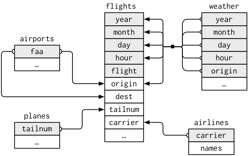
This diagram is a little overwhelming, merely it'southward simple compared to some yous'll see in the wild! The key to understanding diagrams like this is to remember each relation always concerns a pair of tables. You don't need to understand the whole thing; you just need to understand the chain of relations betwixt the tables that you are interested in.
For nycflights13:
-
flightsconnects toplanesvia a unmarried variable,tailnum. -
flightsconnects toairlinesthrough thecarriervariable. -
flightsconnects toairportsin two ways: via theoriginanddestvariables. -
flightsconnects toatmospheric conditionviaorigin(the location), andyear,month,twenty-four hour periodand60 minutes(the time).
Exercises
-
Imagine you wanted to describe (approximately) the route each plane flies from its origin to its destination. What variables would yous demand? What tables would you need to combine?
-
I forgot to depict the relationship betwixt
weatherandairports. What is the relationship and how should information technology appear in the diagram? -
conditionsonly contains information for the origin (NYC) airports. If it contained weather records for all airports in the U.s.a., what additional relation would it define withflights? -
We know that some days of the twelvemonth are "special", and fewer people than usual fly on them. How might you stand for that information as a data frame? What would be the primary keys of that tabular array? How would information technology connect to the existing tables?
Keys
The variables used to connect each pair of tables are called keys. A central is a variable (or set of variables) that uniquely identifies an observation. In simple cases, a single variable is sufficient to identify an observation. For example, each plane is uniquely identified by its tailnum. In other cases, multiple variables may be needed. For case, to identify an observation in weather you demand v variables: year, month, twenty-four hours, hour, and origin.
There are ii types of keys:
-
A chief key uniquely identifies an observation in its own tabular array. For case,
planes$tailnumis a primary cardinal because it uniquely identifies each plane in theplanestable. -
A strange key uniquely identifies an observation in another tabular array. For example,
flights$tailnumis a foreign key because it appears in theflightstable where it matches each flying to a unique plane.
A variable can be both a primary key and a foreign key. For example, origin is role of the weather primary key, and is likewise a foreign key for the airports table.
One time y'all've identified the primary keys in your tables, it'due south good practise to verify that they do indeed uniquely identify each observation. Ane way to do that is to count() the primary keys and expect for entries where north is greater than 1:
planes %>% count ( tailnum ) %>% filter ( n > 1 ) #> # A tibble: 0 x 2 #> # … with 2 variables: tailnum <chr>, n <int> atmospheric condition %>% count ( year, month, day, 60 minutes, origin ) %>% filter ( n > i ) #> # A tibble: three x six #> year month twenty-four hour period hr origin n #> <int> <int> <int> <int> <chr> <int> #> 1 2013 xi 3 1 EWR 2 #> 2 2013 11 three i JFK 2 #> iii 2013 xi 3 1 LGA 2 Sometimes a table doesn't take an explicit primary key: each row is an ascertainment, but no combination of variables reliably identifies information technology. For example, what'south the principal key in the flights table? You might recall it would be the engagement plus the flight or tail number, simply neither of those are unique:
flights %>% count ( year, month, mean solar day, flight ) %>% filter ( n > one ) #> # A tibble: 29,768 10 five #> yr month day flight due north #> <int> <int> <int> <int> <int> #> 1 2013 1 1 one 2 #> 2 2013 1 one 3 2 #> three 2013 1 1 4 two #> iv 2013 i one 11 3 #> 5 2013 one one fifteen two #> 6 2013 1 1 21 two #> # … with 29,762 more than rows flights %>% count ( yr, month, day, tailnum ) %>% filter ( northward > 1 ) #> # A tibble: 64,928 10 5 #> twelvemonth month solar day tailnum n #> <int> <int> <int> <chr> <int> #> one 2013 i one N0EGMQ 2 #> 2 2013 one i N11189 two #> three 2013 one ane N11536 2 #> four 2013 one ane N11544 3 #> five 2013 1 1 N11551 2 #> vi 2013 ane 1 N12540 ii #> # … with 64,922 more than rows When starting to work with this information, I had naively assumed that each flight number would be just used once per twenty-four hours: that would make it much easier to communicate problems with a specific flight. Unfortunately that is non the case! If a tabular array lacks a primary fundamental, it'due south sometimes useful to add together i with mutate() and row_number(). That makes it easier to match observations if you've done some filtering and desire to check back in with the original data. This is called a surrogate central.
A main primal and the corresponding foreign key in another tabular array form a relation. Relations are typically ane-to-many. For example, each flight has one plane, but each plane has many flights. In other data, you lot'll occasionally encounter a 1-to-1 relationship. Yous tin call up of this every bit a special case of 1-to-many. You can model many-to-many relations with a many-to-1 relation plus a ane-to-many relation. For example, in this data in that location's a many-to-many relationship between airlines and airports: each airline flies to many airports; each airport hosts many airlines.
Exercises
-
Add a surrogate key to
flights. -
Identify the keys in the following datasets
-
Lahman::Batting, -
babynames::babynames -
nasaweather::atmos -
fueleconomy::vehicles -
ggplot2::diamonds
(You might demand to install some packages and read some documentation.)
-
-
Draw a diagram illustrating the connections between the
Batting,People, andSalariestables in the Lahman package. Draw another diagram that shows the human relationship betweenPeople,Managers,AwardsManagers.How would you characterise the relationship between the
Batting,Pitching, andFieldingtables?
Mutating joins
The first tool we'll look at for combining a pair of tables is the mutating join. A mutating join allows you to combine variables from 2 tables. Information technology start matches observations by their keys, then copies across variables from one table to the other.
Like mutate(), the join functions add variables to the right, so if yous have a lot of variables already, the new variables won't become printed out. For these examples, we'll arrive easier to come across what's going on in the examples past creating a narrower dataset:
flights2 <- flights %>% select ( yr : day, 60 minutes, origin, dest, tailnum, carrier ) flights2 #> # A tibble: 336,776 10 8 #> year calendar month day hour origin dest tailnum carrier #> <int> <int> <int> <dbl> <chr> <chr> <chr> <chr> #> 1 2013 ane 1 v EWR IAH N14228 UA #> 2 2013 i 1 5 LGA IAH N24211 UA #> iii 2013 i 1 5 JFK MIA N619AA AA #> four 2013 1 1 5 JFK BQN N804JB B6 #> 5 2013 one 1 6 LGA ATL N668DN DL #> 6 2013 1 1 5 EWR ORD N39463 UA #> # … with 336,770 more rows (Call up, when you lot're in RStudio, yous can likewise use View() to avoid this problem.)
Imagine you want to add the full airline name to the flights2 data. Y'all can combine the airlines and flights2 data frames with left_join():
flights2 %>% select ( - origin, - dest ) %>% left_join ( airlines, by = "carrier" ) #> # A tibble: 336,776 x 7 #> year month day hour tailnum carrier proper name #> <int> <int> <int> <dbl> <chr> <chr> <chr> #> i 2013 1 1 5 N14228 UA United Air Lines Inc. #> 2 2013 one 1 v N24211 UA United Air Lines Inc. #> iii 2013 one 1 5 N619AA AA American Airlines Inc. #> 4 2013 1 1 5 N804JB B6 JetBlue Airways #> 5 2013 one ane 6 N668DN DL Delta Air Lines Inc. #> vi 2013 1 1 5 N39463 UA United Air Lines Inc. #> # … with 336,770 more rows The effect of joining airlines to flights2 is an boosted variable: proper noun. This is why I call this blazon of join a mutating join. In this case, you could have got to the aforementioned place using mutate() and R's base subsetting:
flights2 %>% select ( - origin, - dest ) %>% mutate (name = airlines $ name [ match ( carrier, airlines $ carrier ) ] ) #> # A tibble: 336,776 x 7 #> twelvemonth calendar month twenty-four hour period hour tailnum carrier name #> <int> <int> <int> <dbl> <chr> <chr> <chr> #> one 2013 1 1 5 N14228 UA United Air Lines Inc. #> 2 2013 1 1 5 N24211 UA United Air Lines Inc. #> three 2013 1 1 5 N619AA AA American Airlines Inc. #> iv 2013 i 1 5 N804JB B6 JetBlue Airways #> 5 2013 1 ane 6 N668DN DL Delta Air Lines Inc. #> 6 2013 1 1 5 N39463 UA United Air Lines Inc. #> # … with 336,770 more rows Merely this is hard to generalise when y'all need to lucifer multiple variables, and takes shut reading to figure out the overall intent.
The following sections explain, in item, how mutating joins piece of work. Yous'll kickoff past learning a useful visual representation of joins. We'll then use that to explicate the four mutating bring together functions: the inner join, and the 3 outer joins. When working with real data, keys don't always uniquely identify observations, then next we'll talk about what happens when there isn't a unique match. Finally, you'll learn how to tell dplyr which variables are the keys for a given bring together.
Agreement joins
To help you learn how joins work, I'm going to apply a visual representation:
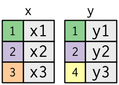
10 <- tribble ( ~ key, ~ val_x, 1, "x1", 2, "x2", iii, "x3" ) y <- tribble ( ~ key, ~ val_y, 1, "y1", two, "y2", 4, "y3" ) The coloured column represents the "key" variable: these are used to match the rows between the tables. The grey column represents the "value" column that is carried along for the ride. In these examples I'll testify a unmarried central variable, but the idea generalises in a straightforward manner to multiple keys and multiple values.
A join is a way of connecting each row in x to goose egg, one, or more rows in y. The following diagram shows each potential match as an intersection of a pair of lines.
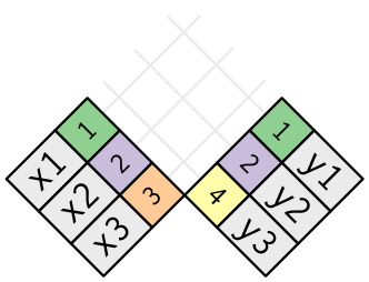
(If you look closely, y'all might notice that we've switched the order of the key and value columns in x. This is to emphasise that joins match based on the key; the value is just carried along for the ride.)
In an actual bring together, matches volition be indicated with dots. The number of dots = the number of matches = the number of rows in the output.
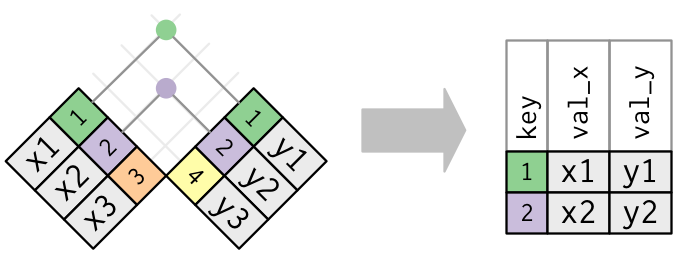
Inner bring together
The simplest type of bring together is the inner bring together. An inner bring together matches pairs of observations whenever their keys are equal:
(To be precise, this is an inner equijoin because the keys are matched using the equality operator. Since nearly joins are equijoins we usually drop that specification.)
The output of an inner join is a new data frame that contains the fundamental, the x values, and the y values. We utilise by to tell dplyr which variable is the key:
x %>% inner_join ( y, by = "key" ) #> # A tibble: 2 10 3 #> key val_x val_y #> <dbl> <chr> <chr> #> 1 ane x1 y1 #> 2 2 x2 y2 The almost important belongings of an inner join is that unmatched rows are non included in the result. This means that generally inner joins are ordinarily not appropriate for employ in analysis because it's besides easy to lose observations.
Outer joins
An inner join keeps observations that appear in both tables. An outer join keeps observations that appear in at to the lowest degree one of the tables. In that location are iii types of outer joins:
- A left join keeps all observations in
x. - A right bring together keeps all observations in
y. - A total bring together keeps all observations in
xandy.
These joins work past adding an additional "virtual" observation to each table. This observation has a primal that always matches (if no other fundamental matches), and a value filled with NA.
Graphically, that looks like:
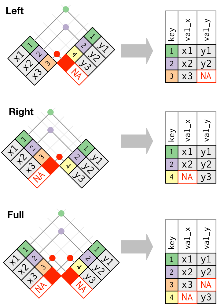
The most normally used bring together is the left join: you lot use this whenever y'all wait upwardly additional information from some other table, because it preserves the original observations even when at that place isn't a match. The left bring together should be your default bring together: use it unless you lot take a stiff reason to adopt 1 of the others.
Another way to describe the dissimilar types of joins is with a Venn diagram:
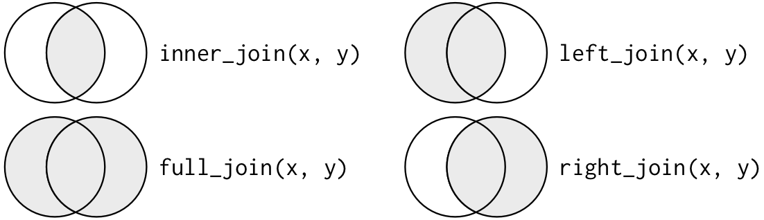
However, this is not a bang-up representation. It might jog your memory about which join preserves the observations in which table, but it suffers from a major limitation: a Venn diagram can't show what happens when keys don't uniquely identify an observation.
Indistinguishable keys
So far all the diagrams accept assumed that the keys are unique. Only that's non always the instance. This section explains what happens when the keys are non unique. There are two possibilities:
-
One table has indistinguishable keys. This is useful when yous desire to add in additional data as there is typically a one-to-many human relationship.
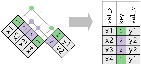
Notation that I've put the central column in a slightly different position in the output. This reflects that the fundamental is a primary key in
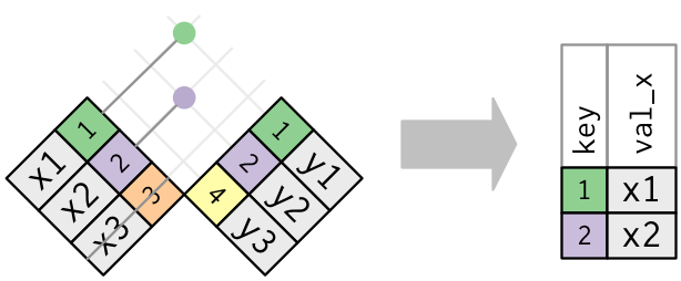
yand a foreign key inx.x <- tribble ( ~ primal, ~ val_x, i, "x1", 2, "x2", 2, "x3", ane, "x4" ) y <- tribble ( ~ key, ~ val_y, i, "y1", 2, "y2" ) left_join ( 10, y, by = "key" ) #> # A tibble: 4 x iii #> key val_x val_y #> <dbl> <chr> <chr> #> ane 1 x1 y1 #> two 2 x2 y2 #> three 2 x3 y2 #> iv 1 x4 y1 -
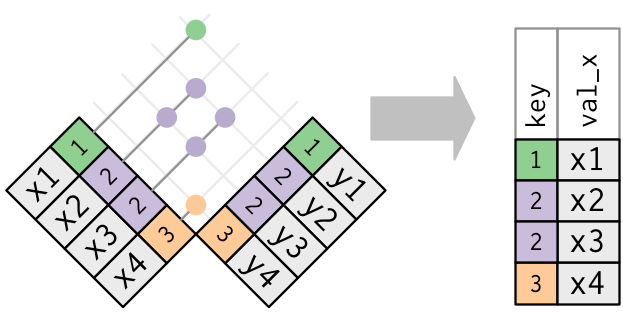
Both tables take duplicate keys. This is usually an error because in neither table exercise the keys uniquely identify an observation. When you bring together duplicated keys, y'all get all possible combinations, the Cartesian product:
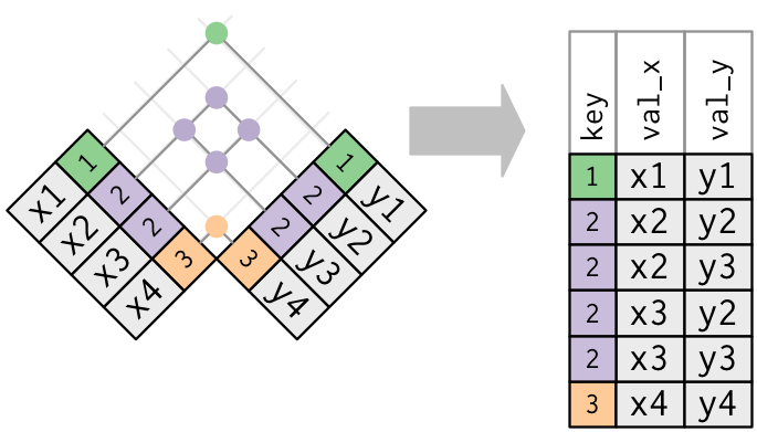
10 <- tribble ( ~ key, ~ val_x, 1, "x1", 2, "x2", 2, "x3", three, "x4" ) y <- tribble ( ~ key, ~ val_y, i, "y1", 2, "y2", 2, "y3", 3, "y4" ) left_join ( x, y, by = "central" ) #> # A tibble: 6 x 3 #> key val_x val_y #> <dbl> <chr> <chr> #> 1 1 x1 y1 #> two 2 x2 y2 #> three two x2 y3 #> four ii x3 y2 #> five 2 x3 y3 #> 6 three x4 y4
Defining the key columns
So far, the pairs of tables accept ever been joined by a unmarried variable, and that variable has the aforementioned proper noun in both tables. That constraint was encoded past past = "key". You lot tin use other values for past to connect the tables in other means:
-
The default,
past = NULL, uses all variables that appear in both tables, the so chosen natural join. For example, the flights and weather condition tables friction match on their common variables:year,month,day,hourandorigin.flights2 %>% left_join ( weather ) #> Joining, by = c("year", "calendar month", "twenty-four hours", "60 minutes", "origin") #> # A tibble: 336,776 ten xviii #> yr month day hr origin dest tailnum carrier temp dewp humid #> <int> <int> <int> <dbl> <chr> <chr> <chr> <chr> <dbl> <dbl> <dbl> #> 1 2013 1 1 v EWR IAH N14228 UA 39.0 28.0 64.4 #> two 2013 1 1 5 LGA IAH N24211 UA 39.nine 25.0 54.8 #> iii 2013 1 1 5 JFK MIA N619AA AA 39.0 27.0 61.half dozen #> 4 2013 i 1 v JFK BQN N804JB B6 39.0 27.0 61.6 #> 5 2013 1 1 6 LGA ATL N668DN DL 39.ix 25.0 54.8 #> 6 2013 1 i v EWR ORD N39463 UA 39.0 28.0 64.4 #> # … with 336,770 more rows, and vii more variables: wind_dir <dbl>, #> # wind_speed <dbl>, wind_gust <dbl>, precip <dbl>, pressure <dbl>, #> # visib <dbl>, time_hour <dttm> -
A graphic symbol vector,
by = "x". This is like a natural join, but uses only some of the common variables. For example,flightsandplaneshaveyearvariables, only they mean dissimilar things so we simply want to join bytailnum.flights2 %>% left_join ( planes, past = "tailnum" ) #> # A tibble: 336,776 x sixteen #> yr.10 month day 60 minutes origin dest tailnum carrier year.y type #> <int> <int> <int> <dbl> <chr> <chr> <chr> <chr> <int> <chr> #> one 2013 one 1 5 EWR IAH N14228 UA 1999 Fixe… #> 2 2013 1 1 5 LGA IAH N24211 UA 1998 Fixe… #> three 2013 i i v JFK MIA N619AA AA 1990 Fixe… #> 4 2013 1 ane 5 JFK BQN N804JB B6 2012 Fixe… #> 5 2013 i 1 6 LGA ATL N668DN DL 1991 Fixe… #> 6 2013 one 1 5 EWR ORD N39463 UA 2012 Fixe… #> # … with 336,770 more rows, and half-dozen more than variables: manufacturer <chr>, #> # model <chr>, engines <int>, seats <int>, speed <int>, engine <chr>Note that the
yearvariables (which appear in both input data frames, but are not constrained to be equal) are disambiguated in the output with a suffix. -
A named character vector:
past = c("a" = "b"). This will match variableain tablexto variablebin tabular arrayy. The variables fromxwill be used in the output.For example, if nosotros want to draw a map we demand to combine the flights data with the airports data which contains the location (
latandlon) of each drome. Each flying has an origin and destinationairport, so we need to specify which one we want to join to:flights2 %>% left_join ( airports, c ( "dest" = "faa" ) ) #> # A tibble: 336,776 x xv #> year month day hour origin dest tailnum carrier name lat lon alt #> <int> <int> <int> <dbl> <chr> <chr> <chr> <chr> <chr> <dbl> <dbl> <dbl> #> one 2013 1 1 5 EWR IAH N14228 UA Geor… 30.0 -95.3 97 #> two 2013 1 i 5 LGA IAH N24211 UA Geor… 30.0 -95.3 97 #> 3 2013 1 i five JFK MIA N619AA AA Miam… 25.viii -80.iii 8 #> 4 2013 1 1 five JFK BQN N804JB B6 <NA> NA NA NA #> 5 2013 ane 1 6 LGA ATL N668DN DL Hart… 33.6 -84.4 1026 #> 6 2013 1 1 5 EWR ORD N39463 UA Chic… 42.0 -87.9 668 #> # … with 336,770 more rows, and 3 more than variables: tz <dbl>, dst <chr>, #> # tzone <chr> flights2 %>% left_join ( airports, c ( "origin" = "faa" ) ) #> # A tibble: 336,776 10 15 #> year month day hr origin dest tailnum carrier name lat lon alt #> <int> <int> <int> <dbl> <chr> <chr> <chr> <chr> <chr> <dbl> <dbl> <dbl> #> ane 2013 i 1 5 EWR IAH N14228 UA Newa… forty.vii -74.2 18 #> 2 2013 1 one five LGA IAH N24211 UA La G… 40.eight -73.9 22 #> 3 2013 one ane 5 JFK MIA N619AA AA John… 40.6 -73.8 13 #> 4 2013 1 1 5 JFK BQN N804JB B6 John… 40.6 -73.8 thirteen #> 5 2013 1 1 half dozen LGA ATL N668DN DL La K… forty.8 -73.9 22 #> 6 2013 1 one 5 EWR ORD N39463 UA Newa… 40.7 -74.2 eighteen #> # … with 336,770 more rows, and three more variables: tz <dbl>, dst <chr>, #> # tzone <chr>
Exercises
-
Compute the boilerplate delay by destination, then join on the
airportsinformation frame and then you can show the spatial distribution of delays. Here'southward an easy way to draw a map of the United States:(Don't worry if you don't sympathise what
semi_join()does — you'll acquire about information technology next.)You might desire to use the
sizeorcolourof the points to brandish the average delay for each drome. -
Add the location of the origin and destination (i.e. the
latandlon) toflights. -
Is there a relationship betwixt the age of a plane and its delays?
-
What weather conditions get in more likely to run into a delay?
-
What happened on June 13 2013? Display the spatial pattern of delays, and so apply Google to cantankerous-reference with the weather.
Other implementations
base of operations::merge() tin perform all four types of mutating join:
| dplyr | merge |
|---|---|
inner_join(x, y) | merge(x, y) |
left_join(x, y) | merge(x, y, all.x = True) |
right_join(x, y) | merge(x, y, all.y = TRUE), |
full_join(x, y) | merge(x, y, all.x = Truthful, all.y = True) |
The advantages of the specific dplyr verbs is that they more clearly convey the intent of your lawmaking: the difference between the joins is really important simply concealed in the arguments of merge(). dplyr's joins are considerably faster and don't mess with the order of the rows.
SQL is the inspiration for dplyr's conventions, so the translation is straightforward:
| dplyr | SQL |
|---|---|
inner_join(x, y, by = "z") | SELECT * FROM 10 INNER Join y USING (z) |
left_join(x, y, by = "z") | SELECT * FROM x LEFT OUTER Join y USING (z) |
right_join(x, y, past = "z") | SELECT * FROM x Right OUTER JOIN y USING (z) |
full_join(x, y, by = "z") | SELECT * FROM x Full OUTER Bring together y USING (z) |
Annotation that "INNER" and "OUTER" are optional, and often omitted.
Joining different variables betwixt the tables, e.one thousand.inner_join(x, y, by = c("a" = "b")) uses a slightly different syntax in SQL: SELECT * FROM x INNER Bring together y ON x.a = y.b. As this syntax suggests, SQL supports a wider range of join types than dplyr considering y'all can connect the tables using constraints other than equality (sometimes called non-equijoins).
Filtering joins
Filtering joins friction match observations in the same mode as mutating joins, but bear on the observations, not the variables. At that place are two types:
-
semi_join(ten, y)keeps all observations intenthat have a match iny. -
anti_join(x, y)drops all observations inxthat take a match iny.
Semi-joins are useful for matching filtered summary tables back to the original rows. For example, imagine you've establish the top ten most pop destinations:
top_dest <- flights %>% count ( dest, sort = TRUE ) %>% head ( 10 ) top_dest #> # A tibble: 10 ten two #> dest north #> <chr> <int> #> ane ORD 17283 #> 2 ATL 17215 #> 3 LAX 16174 #> 4 BOS 15508 #> 5 MCO 14082 #> 6 CLT 14064 #> # … with 4 more rows Now you want to discover each flight that went to one of those destinations. You could construct a filter yourself:
flights %>% filter ( dest %in% top_dest $ dest ) #> # A tibble: 141,145 x xix #> year calendar month twenty-four hour period dep_time sched_dep_time dep_delay arr_time sched_arr_time #> <int> <int> <int> <int> <int> <dbl> <int> <int> #> i 2013 1 1 542 540 2 923 850 #> 2 2013 1 1 554 600 -6 812 837 #> 3 2013 i 1 554 558 -4 740 728 #> four 2013 one ane 555 600 -5 913 854 #> five 2013 i one 557 600 -3 838 846 #> 6 2013 ane 1 558 600 -2 753 745 #> # … with 141,139 more than rows, and 11 more variables: arr_delay <dbl>, #> # carrier <chr>, flight <int>, tailnum <chr>, origin <chr>, dest <chr>, #> # air_time <dbl>, distance <dbl>, hour <dbl>, minute <dbl>, time_hour <dttm> Just it'southward difficult to extend that arroyo to multiple variables. For example, imagine that you'd plant the 10 days with highest average delays. How would you construct the filter statement that used year, month, and solar day to match it back to flights?
Instead you can utilize a semi-join, which connects the ii tables like a mutating join, just instead of adding new columns, merely keeps the rows in x that have a match in y:
flights %>% semi_join ( top_dest ) #> Joining, past = "dest" #> # A tibble: 141,145 x xix #> yr calendar month day dep_time sched_dep_time dep_delay arr_time sched_arr_time #> <int> <int> <int> <int> <int> <dbl> <int> <int> #> 1 2013 1 1 542 540 2 923 850 #> 2 2013 1 1 554 600 -6 812 837 #> three 2013 one 1 554 558 -4 740 728 #> iv 2013 1 1 555 600 -5 913 854 #> 5 2013 1 1 557 600 -iii 838 846 #> six 2013 1 1 558 600 -2 753 745 #> # … with 141,139 more than rows, and 11 more than variables: arr_delay <dbl>, #> # carrier <chr>, flight <int>, tailnum <chr>, origin <chr>, dest <chr>, #> # air_time <dbl>, distance <dbl>, hour <dbl>, minute <dbl>, time_hour <dttm> Graphically, a semi-join looks like this:
Only the being of a friction match is of import; it doesn't thing which observation is matched. This means that filtering joins never duplicate rows similar mutating joins do:
The inverse of a semi-join is an anti-bring together. An anti-join keeps the rows that don't accept a match:
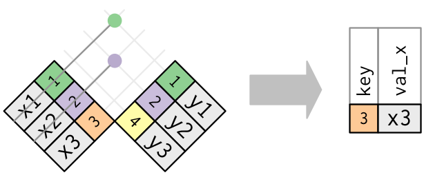
Anti-joins are useful for diagnosing join mismatches. For example, when connecting flights and planes, you might be interested to know that in that location are many flights that don't have a match in planes:
flights %>% anti_join ( planes, past = "tailnum" ) %>% count ( tailnum, sort = TRUE ) #> # A tibble: 722 ten ii #> tailnum n #> <chr> <int> #> i <NA> 2512 #> 2 N725MQ 575 #> iii N722MQ 513 #> iv N723MQ 507 #> 5 N713MQ 483 #> 6 N735MQ 396 #> # … with 716 more rows Exercises
-
What does it mean for a flight to have a missing
tailnum? What practise the tail numbers that don't take a matching record inplaneshave in common? (Hint: one variable explains ~90% of the issues.) -
Filter flights to only show flights with planes that have flown at least 100 flights.
-
Combine
fueleconomy::vehiclesandfueleconomy::commonto find only the records for the about common models. -
Observe the 48 hours (over the course of the whole yr) that have the worst delays. Cross-reference it with the
weatherdata. Can you see whatsoever patterns? -
What does
anti_join(flights, airports, by = c("dest" = "faa"))tell you? What doesanti_join(airports, flights, by = c("faa" = "dest"))tell you lot? -
You might wait that at that place's an implicit human relationship betwixt airplane and airline, considering each plane is flown past a single airline. Confirm or pass up this hypothesis using the tools yous've learned above.
Join problems
The data y'all've been working with in this affiliate has been cleaned up and then that yous'll have as few problems every bit possible. Your own data is unlikely to be so dainty, so there are a few things that you should do with your own information to make your joins become smoothly.
-
Outset by identifying the variables that form the primary cardinal in each tabular array. You should usually practice this based on your understanding of the data, not empirically by looking for a combination of variables that give a unique identifier. If yous just look for variables without thinking nigh what they mean, you might get (united nations)lucky and find a combination that'southward unique in your electric current information merely the relationship might not be true in full general.
For instance, the distance and longitude uniquely identify each drome, but they are not good identifiers!
airports %>% count ( alt, lon ) %>% filter ( northward > 1 ) #> # A tibble: 0 x 3 #> # … with iii variables: alt <dbl>, lon <dbl>, n <int> -
Check that none of the variables in the chief central are missing. If a value is missing and so it tin can't identify an observation!
-
Check that your strange keys friction match primary keys in some other table. The best way to do this is with an
anti_join(). It'due south common for keys not to friction match considering of information entry errors. Fixing these is often a lot of piece of work.If you lot exercise have missing keys, you'll need to be thoughtful about your utilise of inner vs. outer joins, carefully considering whether or not you want to drop rows that don't accept a match.
Be aware that simply checking the number of rows earlier and after the bring together is not sufficient to ensure that your join has gone smoothly. If yous have an inner join with duplicate keys in both tables, y'all might become unlucky equally the number of dropped rows might exactly equal the number of duplicated rows!
Set operations
The final type of two-tabular array verb are the set operations. Generally, I use these the least frequently, just they are occasionally useful when you want to break a single complex filter into simpler pieces. All these operations piece of work with a complete row, comparing the values of every variable. These expect the x and y inputs to have the aforementioned variables, and treat the observations similar sets:
-
intersect(x, y): return simply observations in bothxandy. -
union(x, y): return unique observations inxandy. -
setdiff(ten, y): render observations in10, simply not iny.
Given this uncomplicated information:
df1 <- tribble ( ~ x, ~ y, 1, 1, 2, 1 ) df2 <- tribble ( ~ x, ~ y, 1, ane, 1, two ) The four possibilities are:
intersect ( df1, df2 ) #> # A tibble: 1 ten 2 #> x y #> <dbl> <dbl> #> 1 one 1 # Notation that we get 3 rows, not 4 marriage ( df1, df2 ) #> # A tibble: 3 x two #> x y #> <dbl> <dbl> #> one ane ane #> ii 2 one #> 3 one ii setdiff ( df1, df2 ) #> # A tibble: ane x 2 #> x y #> <dbl> <dbl> #> 1 2 1 setdiff ( df2, df1 ) #> # A tibble: i ten 2 #> ten y #> <dbl> <dbl> #> 1 ane 2 
What Is A Data Table In Science,
Source: https://r4ds.had.co.nz/relational-data.html
Posted by: haidereverporly.blogspot.com
0 Response to "What Is A Data Table In Science"
Post a Comment